Alternate Rows and Columns Shading in Microsoft Excel Using Conditional Formatting

In Microsoft Excel, you can easily format the table by using conditional formatting. By using alternate row or columns shading you can make your worksheet user friendly.

In this post you will learn how to apply conditional formatting for alternate rows or columns shading in Excel. Shading automatically updated, if you add or delete rows or columns within the conditional formatting.

By following below mentioned steps you can easily apply Alternate shading:

Step 1: Select your desired range for formatting.

Step 2: Now Click Home and then in Style group, Click on Conditional Formatting.

Step 3: In Conditional Formatting tab, Click on New Rule to open Formatting Rule dialog box.

Step 4: In Formatting Rule dialog box, In Rule Type, select "Use a Formula to Determine Which Cells to Format".

Step 5: Now enter the below mentioned formula in Format Values Where This Formulas is True.

=MOD(ROW(),2)=0

Step 6: Now Click on Format Button to open Format Cells dialog box as mentioned below:

Step 7: Now in the Format Cells dialog box, Click the Fill tab and select a background fill color and Click OK.

Step 8: Again click OK to close the New Formatting Rule dialog box.

Now you can see the result as mentioned below:

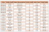
You can also use another format like Checkerboard shading by using below mentioned formula in Format Values Where This Formulas is True.

=MOD(ROW(),2)=MOD(COLUMN(),2)

Now you can see the result as mentioned below:

---Thank You---